Pivot-ing Data

Pivot as a noun is defined by Encarta Dictionary as Crucial Person or Thing : somebody or something that is essential to the success or effectiveness of an activity or event

Surely, Pivots can be used to summarize huge chunks of data with an inherent advantage of dynamic views. The data can reside within a worksheet or an external source.

We shall delve into some features while doing the exercise.

You can download the below excel file to play with pivots. Hit the download button in the top bar.

 

Download Exercise here

 

 

(1) CREATE A PIVOT

As you can observe, the table contains various orders of sales persons along with order details and territory country. For example Buchanan’s territory is UK and he has a order on 16-July-2003 with an unique order ID#10248 amounting to $ 440.

We might like to have a look at total sales made by Buchanan in UK and compare it with Dodsworth.

(1.1) Select the entire table by placing the cursor box in cell A1 and with CTRL + SHIFT pressed, hit the DOWN ↓ arrow once and then the RIGHT → arrow once. This selects the entire data.

(1.2) Go to INSERT tab and select PivotTable. The range would be already reflected in the selection box. Keep NEW WORKSHEET radio button ‘marked’ and then press OK.

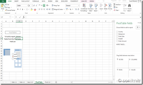
(1.3) You will end up with a new sheet & a blank table as shown below:

(1.3.1) Drag the Order Amount field in the ∑VALUES Area. Click the “Sum of Order…” in values section at bottom right and go to value field settings. Make sure “Sum” is selected and click OK.

 

 

If the fields are somehow hidden, you can place the cursor on any part of the pivot table → Select Analyze Tab → And then activate Field List as shown below

(1.3.2) Drag Country field into COLUMNS Area and Salesperson field into ROWS Area.

With some design in the DESIGN tab and by selecting the comma operator for all the data in the pivot table, you will get a summary as shown.

Salespersons belonging to UK or US have their total sales summarized under their respective country/territory.

Since Buchanan takes care of UK, he will not make any sale under US.

(1.3.3) We can also put a pivot chart from INSERT tab by selecting PivotChart → PivotChart → OK as shown below

The chart is customizable on deck & colour levels and more importantly it is dynamic with your PivotTable. Try dragging Country field from COLUMNS Area into ROWS Area to see how it changes.

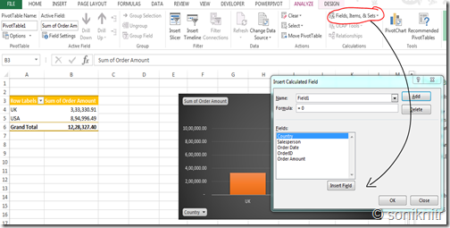
(1.3.4) Let’s say you need to calculate the country tax on total order amount, for sake of simplicity) and take the tax rate as 35%. (actually for US it’s around 40% and for UK it’s 21%)

You can take the Country field into ROWS Area and remove the Salesperson field by dragging it outside the 4 Areas.
To remove a field simply uncheck the field in PivotTable Fields OR drag it from the Areas to anywhere outside

To add a tax calculation field go to → ANALYZE tab → Field, Item & Sets → Calculated Field.

• Enter “Tax” as Name of the field → in Formula enter “= 35% *
• Now choose Order Amount from Fields → click Insert Field
• OK

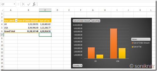
Now you would be able to see the Tax payable as below both in the Table and Chart

You can use calculated formulas with all basic operators like +, –, /, *.

For filtering data in a PivotTable you can drag a field into FILTER Area and drop down to select relevant items in the table (Selection of Multiple Items can be checked)