Basic Arithmetic Operations

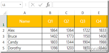
In this post, we review some basic spreadsheet arithmetic along with some flavour of in-cell graphics. Let’s take the quarterly sales data of your prime salespeople namely Alex, Bruce, Candy & Dorothy and look at how we would like to incentivize them to keep it rolling.

You might create the below table in your worksheet.

If they are the only sales people in your company, you might need to look at overall sales of your company for a quarter.

(1) So building on the above table we would like to get some basic arithmetic in place.
^Syntax = SUM(Start Cell:End Cell)

You can replace SUM with COUNT, AVERAGE, MAX or MIN to get the required result.

COUNTA calculates the number of non-empty cells.

(2) Now if you want to find out what was the 2nd highest or 3rd lowest sale of that particular quarter, MAX or MIN would not work. The functions to use would be SMALL or LARGE.

^Syntax = SMALL(Start Cell:End Cell, Index number)  Replace SMALL with LARGE

Since we have only 4 salespersons the 2nd maximum and the 3rd minimum will be the same.

Let’s have a look.

Now if I wish to have the formula replicated over the entire table, I would just drag the handle, seen as a black square at the bottom right corner when I select cells B6 : B12. If the handle is not visible you may either copy paste the entire range till F12 else go to Excel Options from either Office Logo (Top-left corner – 2010) or File (2013) and select the Enable fill handle from Advanced.

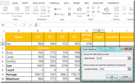
(3) We can have some visual add-in to check the trend in a single cell. These are called sparklines and they come in Insert Tab (Office 2010 onwards).

It will ask for a range for which we would select Alex’s sales data from Q1 to Q4. And the output would be cell H2, which would come automatically if your cursor is present there before insert action.

Alternatively you can also insert a line graph in another cell. You can highlight the high and low points and select custom marker colours for high and low in the DESIGN tab.

(4) For incentive calculation, let us have a rule that the minimum sales per quarter should be more than 1300 to get any incentive.

And incentive can be 10% of total sales if the condition is met.

So, how do we formulate the incentive with functions we already know ?

Here is an example with the IF condition:

(5) Now you wish to award an additional bonus of 1000, if the sales per quarter has exceeded 1300 and total annual sales is more than 6500 for your salesperson.

That’s it for today. Have a good night.