Pivot-ing Data

Pivot as a noun is defined by Encarta Dictionary as Crucial Person or Thing : somebody or something that is essential to the success or effectiveness of an activity or event

Surely, Pivots can be used to summarize huge chunks of data with an inherent advantage of dynamic views. The data can reside within a worksheet or an external source.

We shall delve into some features while doing the exercise.

You can download the below excel file to play with pivots. Hit the download button in the top bar.

 

Download Exercise here

 

 

(1) CREATE A PIVOT

As you can observe, the table contains various orders of sales persons along with order details and territory country. For example Buchanan’s territory is UK and he has a order on 16-July-2003 with an unique order ID#10248 amounting to $ 440.

We might like to have a look at total sales made by Buchanan in UK and compare it with Dodsworth.

(1.1) Select the entire table by placing the cursor box in cell A1 and with CTRL + SHIFT pressed, hit the DOWN ↓ arrow once and then the RIGHT → arrow once. This selects the entire data.

(1.2) Go to INSERT tab and select PivotTable. The range would be already reflected in the selection box. Keep NEW WORKSHEET radio button ‘marked’ and then press OK.

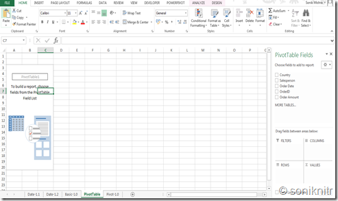
(1.3) You will end up with a new sheet & a blank table as shown below:

(1.3.1) Drag the Order Amount field in the ∑VALUES Area. Click the “Sum of Order…” in values section at bottom right and go to value field settings. Make sure “Sum” is selected and click OK.

 

 

If the fields are somehow hidden, you can place the cursor on any part of the pivot table → Select Analyze Tab → And then activate Field List as shown below

(1.3.2) Drag Country field into COLUMNS Area and Salesperson field into ROWS Area.

With some design in the DESIGN tab and by selecting the comma operator for all the data in the pivot table, you will get a summary as shown.

Salespersons belonging to UK or US have their total sales summarized under their respective country/territory.

Since Buchanan takes care of UK, he will not make any sale under US.

(1.3.3) We can also put a pivot chart from INSERT tab by selecting PivotChart → PivotChart → OK as shown below

The chart is customizable on deck & colour levels and more importantly it is dynamic with your PivotTable. Try dragging Country field from COLUMNS Area into ROWS Area to see how it changes.

(1.3.4) Let’s say you need to calculate the country tax on total order amount, for sake of simplicity) and take the tax rate as 35%. (actually for US it’s around 40% and for UK it’s 21%)

You can take the Country field into ROWS Area and remove the Salesperson field by dragging it outside the 4 Areas.
To remove a field simply uncheck the field in PivotTable Fields OR drag it from the Areas to anywhere outside

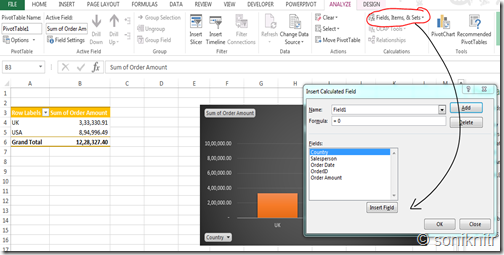
To add a tax calculation field go to → ANALYZE tab → Field, Item & Sets → Calculated Field.

• Enter “Tax” as Name of the field → in Formula enter “= 35% *
• Now choose Order Amount from Fields → click Insert Field
• OK

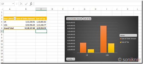
Now you would be able to see the Tax payable as below both in the Table and Chart

You can use calculated formulas with all basic operators like +, –, /, *.

For filtering data in a PivotTable you can drag a field into FILTER Area and drop down to select relevant items in the table (Selection of Multiple Items can be checked)

Basic Arithmetic Operations

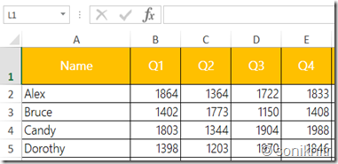
In this post, we review some basic spreadsheet arithmetic along with some flavour of in-cell graphics. Let’s take the quarterly sales data of your prime salespeople namely Alex, Bruce, Candy & Dorothy and look at how we would like to incentivize them to keep it rolling.

You might create the below table in your worksheet.

If they are the only sales people in your company, you might need to look at overall sales of your company for a quarter.

(1) So building on the above table we would like to get some basic arithmetic in place.
^Syntax = SUM(Start Cell:End Cell)

You can replace SUM with COUNT, AVERAGE, MAX or MIN to get the required result.

COUNTA calculates the number of non-empty cells.

(2) Now if you want to find out what was the 2nd highest or 3rd lowest sale of that particular quarter, MAX or MIN would not work. The functions to use would be SMALL or LARGE.

^Syntax = SMALL(Start Cell:End Cell, Index number)  Replace SMALL with LARGE

Since we have only 4 salespersons the 2nd maximum and the 3rd minimum will be the same.

Let’s have a look.

Now if I wish to have the formula replicated over the entire table, I would just drag the handle, seen as a black square at the bottom right corner when I select cells B6 : B12. If the handle is not visible you may either copy paste the entire range till F12 else go to Excel Options from either Office Logo (Top-left corner – 2010) or File (2013) and select the Enable fill handle from Advanced.

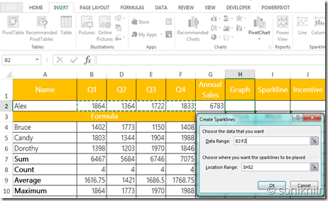
(3) We can have some visual add-in to check the trend in a single cell. These are called sparklines and they come in Insert Tab (Office 2010 onwards).

It will ask for a range for which we would select Alex’s sales data from Q1 to Q4. And the output would be cell H2, which would come automatically if your cursor is present there before insert action.

Alternatively you can also insert a line graph in another cell. You can highlight the high and low points and select custom marker colours for high and low in the DESIGN tab.

(4) For incentive calculation, let us have a rule that the minimum sales per quarter should be more than 1300 to get any incentive.

And incentive can be 10% of total sales if the condition is met.

So, how do we formulate the incentive with functions we already know ?

Here is an example with the IF condition:

(5) Now you wish to award an additional bonus of 1000, if the sales per quarter has exceeded 1300 and total annual sales is more than 6500 for your salesperson.

That’s it for today. Have a good night.

Basic Date Arithmetic

You would have come across data with dates and sometimes you would have needed to get a corresponding date or day after a certain period of time. For example, a confirmation date after 6 months or a date post payment terms of 90 days or post an ageing schedule for 6 months.

Please refer this post for Date basics

We shall take up this exercise in a common template which is given below. It will take just a few seconds to type in.

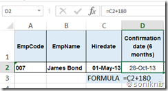
Case 1) Employee 007 has joined your organization on 01-May-2013. We need to find his date of confirmation after a period of six months {in the cell D2}

An easier but more approximate method would be directly add the number of days in D2.

6 months ~ 180 days

^Syntax = D2 = C2 + 180

However, it’s an approximation as each of the months succeeding May-2013 would not have exactly 30 days.

^*If the cell is not in a format that displays a date, you can right-click on the cell and format cell as date.

(Refer this post in case of any doubts)

 

Case 2) 2a) Alternatively, we can use a formula called EDATE, which would correctly add up the six following months after 01-May-2013

^Syntax = EDATE(Start Date or Input Date, Number of Months)

Use of EDATE with inputs as previous cell and 6 months gives the desired result.

So, Mr. Bond should have been confirmed on 01-Nov-2013, we may need to check out if it’s a working day or not. You would not like to give a confirmation letter to Mr. Bond on a Sunday, right?

2b) Let’s find out the day of the week for that purpose.

^Syntax = WEEKDAY(Input Date or D2, Return type usually as 1)

• For our calendar & context, we use 1 as the return type since our week usually starts on a Sunday (=1) and ends on a Saturday (=7).
• Now when we get the result, it pops out as a serial number i.e 6 in this case.
• For that we need an already familiar function called TEXT() (Described in this post) with the required parameters, which would be the WEEKDAY input and formatting for returning the full day name i.e “dddd” (more than 3 d’s, 3 d’s will return a short day name, 2 d’s the serial number)

2c) DATEDIFFERENCE This case refers to a situation in which need to find the time for which James Bond has served your organization.

There is a MS-undocumented function which historically is borrowed by Microsoft from a company called, well it’s Lotus (now owned by IBM). So, it will never show the arguments for an input although a small popup surfaces, when you type DATEDIF(

 

^Syntax = DATEDIF(Start Date, End Date, Unit of Formatting)

Units of Formatting

^DF.Syntax Y – Number of compete Years

^DF.Syntax M – Number of compete Months

^DF.Syntax D – Number of Days

^DF.Syntax YM – Number of complete Months after subtracting the completed years. (< 12) (Days not summing to 1 month are ignored)

^DF.Syntax MD – Number of Days after subtracting the completed months & years

^DF.Syntax YD – Number of Days after subtracting the completed years (months included)

If you take the start date of our James Bond, and dynamic function - TODAY()  as the end date taking the M argument gives the following result.

Exercise

Now applying the same principles can you get an output of Total Experience like the one in the bottom-right cell ? (You may do a search on text operators)

Have a nice weekend folks!

The Date Function

If you have ever come across loads of data in a spreadsheet involving dates or inventory ageing, you have probably come across some of the things described below. We will wade through these common scenarios and applications one by one. Some of the formulas used in this context might seem unique or rather a little crazy while others may seem quite generic. We will take up the not so unfamiliar DATE functionality in this post.

And you may have possibilities that outperform the ones described here. Please feel free to use the comments section for that purpose.

 

Now to the DATE function : Microsoft defines it as unique sequential serial number that returns on a particular date.

^Syntax = DATE(Year, Month, Day)

You may write 30-August-2014 as DATE(2014, 8, 30) and if you change the date format to a number format it should give 41881.00^[1]

 

 

 

 

1.1) When does this function help ?

You may have at times encountered data in which dates are not in a ‘excel recognizable’ format in cases like downloads from ERP software, internet banking or text dumps in CSV formats among others. And Data –> text to columns for a date format might not work on them.

 

And in many such cases you would have experienced that selecting the format as date dropdown doesn’t work as seen in the below image. It might be quite tedious to correct multiple dates, and that’s exactly where DATE as a function comes in handy.

 

1.2) How ?

1.2.1 - We use some text functions mainly LEFT, RIGHT & MID to extract the necessary strings.

 

^Syntax = LEFT(Select Text Cell, number of characters to be extracted from Left)

^Syntax = RIGHT(Select Text Cell, number of characters to be extracted from Right)

^Syntax = MID(Select Text Cell, Start number for 1st character to be extracted from Left, number of characters to be extracted after that)

 

Using the text formulas nested within the DATE function we can extract the required date and consequently we can use it to do things like DATE ARITHMETIC – Add, Subtract, Find Difference, Find the Calendar Day or next working day among others, which shall be discussing in another post.

 

1.3) I want to have it in another format. How do I do that?

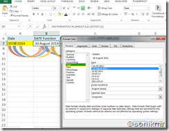
One, if you want to have a different format such as MM/DD/YYY or a standard format in the same cell you can right-click on the cell A7 and select Format Cells and navigate to Date in the side tab as shown here.

Alternatively, you can drop down the number formatting tab and select ‘More Number formats’.

For a custom format, one can choose custom from the left pane and type in the required date formatting syntax.

 

^DF.Syntax DD – Numerical Date

^DF.Syntax DDD – Day (Monday, Tuesday…)

^DF.Syntax MM – Numerical Month (01-January, 02- February…)

^DF.Syntax MMM – First three letters of the name of the month (Jan – January)

^DF.Syntax MMMM – Complete name of the Month

^DF.Syntax YY – Last two digit of the year

^DF.Syntax YYY – Complete year

 

1.3.1) If you wish to take a specific formatting for display only purpose to another cell then you may use the TEXT function. However, date operations or algebra (we shall take it up in a later post) will not be possible for a text output.

^Syntax = TEXT(Select Reference Cell, “Required formatting within double quotes”)

Formatting for the date should be kept within double quotes with the DF.Syntax i.e date formatting syntaxes discussed above.

 

1.4) What if I enter day, month beyond the normal range of 31 and 12, or negative values.
Excel would subtract (negative days/months) or add (beyond 30 or 31 days, 12 months) from the entered date and give the final date.
Here it takes 31 days for August and adds the rest 14 days to hop to 14-September.
[1] As it stores date starting with 01-Jan-1900 as 1. So negative arguments will give erroneous results if calculation takes the date prior to the year 1900.

1.5) TODAY() gives today’s date as in the computer. It’s dynamic and will change everyday.
^Syntax = TODAY()